Today’s post is about a subject I presented a few years back at the entrance exams of the french engineering schools. If you like clocks, boats, adventures and unnecessary complications, this is for you 🙂
Historical notice
During the Renaissance the English realised how good they were on seas, and how much potential there was for some ass-kicking with all these loaded European ships making round trips to America. A very crucial problem in sailing is to know where you are. For that you need
- Your latitude : how far north are you from the equator ?
- Your longitude : how far west are you from London ?
Getting the latitude is easy:
- During the day, look at the sun (especially at noon). The higher it is, the nearer you are from the equator
- At night, look at a pole star : the higher it is, the farther away you are from the equator.
But no such tricks to estimate the longitude existed in the 1700’s. Astronomers had thought of something but it was all very complicated and stuff. So the English did what you do when you are out of ideas: they made a law (the Longitude Act) proposing a huge prize (that they had no intention of giving up too easily) to any subject of his Majesty who would come up first with a method.
That’s were John Harrison comes in, with a beautifully simple idea:
- Take a clock indicating London’s time onboard.
- During your travel, look at the sun to get the time of the place where you are, and compare it to the clock’s time.
- If for instance the sun indicates 12h00, and the clock indicates that it is 10h00 in London, then you know that you are
 degrees west from London.
The only problem is that, if you take your good old pendulum clock on a boat, it will instantly go mad due to all that pitching, rolling and yawing ! So you need to design a more sophisticated device. But John Harrison had a slight advantage here: he was a professional clockmaker !
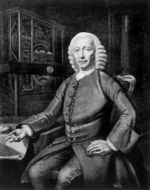
John Harrison (1693-1776) Credit: Wikipedia
Shake it baby ! Harrison’s H1 clock
In 1730, Harrison imagines his first marine clock, that he calls H1:

Harrison’s H1. Credit : National Maritime Museum, (Greenwich)
Here is an idealized scheme of the beast’s arms :

I believe that the contact between the two arms is there to make sure that they will always move in symetrical ways (otherwise the movement could get chaotic). A very nice feature of this design is that any force that is applied equally to each of the weights is cancelled out and has no effect on the oscillations !

This makes the clock’s movement independent from gravity (meaning that the clock doesn’t need to be vertical to oscillate properly) and from any translational movement of the boat !
However (and that’s where my study started) I noticed that the centrifuge force induced by the rolling of the ship is not compensated, as the weights are not equally distant from the rotation center:

And my (very fundamental and of much historical importance) question was : how much does the rolling affect the clock ?
A small study
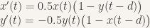
Before getting to the real question, let us study how this clock works when it is not perturbated.
Suppose that the left arm, of radius  makes an angle
  with its equilibrium position (that we suppose to be vertical):

The other arm is in a symetrical position, so the upper spring is streched by a length  and thus pulls the upper weight of the left arm with a force equal to
  (where k is the spring’s rigidity constant). The lower spring is compressed by a length and the lower weight undergoes a push of . These two forces apply negative torques on the arm, both with a lever equal to
  . Finally, neglecting the mass of the arm’s sticks, the arm’s angular momentum is
  where M is the mass of one weight. Once you have all that, the angular momentum theorem gives

which after simplifications gives
Note that (partly because my model is very simple) the oscillations do not depend on the radius of the arms. If the amplitude of the oscillations if really small, we have  and the equation becomes

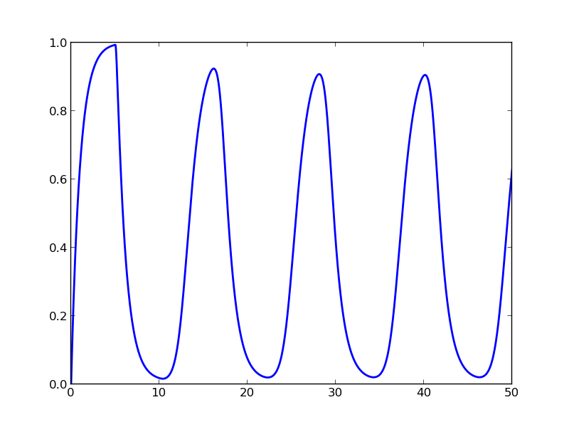
where we recognize an harmonic oscillator of period  . If the oscillations are bigger, one can still simulate the dynamics (here with Python):
from pylab import *
from scipy.integrate import odeint
def H1diff(Y,t,k,M):
"""
Equations describing the dynamics of the model
Y is [A,dA/dt], t is the current time, k is the spring's constant,
M is the mass of the weights.
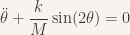
Returns [dA/dt, ddA/ddt] according to
dd(A)/ddt + k/M sin(2A) = 0
"""
A,dA = Y
return array([dA, -k / M * sin(2*A)])
k=1.0 ; M=1.0 ; initialAngle = pi/6 # parameters
Y0= [pi/6, 0.0] # initial angle pi/6, initial speed 0
ts=linspace(0,10, 100) # 100 times points between 0 and 10
angles = odeint(H1diff,[initialAngle,0],ts,args=(k,M))[:,0] # solving
# plotting
fig,ax = subplots(1)
ax.plot(ts,angles) # plotting
ax.set_xlabel('time',fontsize = 24)
ax.set_ylabel('angle',fontsize = 24)
show()

Or better 🙂
def makeAnimation(k=1.0,M=1.0,nframes=40,R=1.0,**kwargs):
    """ simulates and creates a GIF of the H1 """

    # default for tmax is one period.
    tmax = kwargs.pop('tmax',2*pi*sqrt(M/k))

    # delay is computed so that the animation actually lasts tmax.
    delay = kwargs.pop('delay',int(100.0*tmax/nframes))

    O1 = array([-1.0,0]) # center of the left pendulum
    O2 = array([1.0,0])  # center of the right pendulum
    R = 1.0

    def drawH1(angle,ax):
        """ draws an Harrison H1 clock given the angle of the arms """

        # compute the coordinates of the four weights:

        s,c = sin(angle), cos(angle)
        LU = O1 + R*array([-s,c])
        LD = O1 + R*array([s,-c])
        RU = O2 + R*array([s,c])
        RD = O2 + R*array([-s,-c])

        # draw the springs

        for w1,w2 in (LU,RU),(LD,RD):
            ax.add_line(Line2D(*zip(w1,w2), linewidth=2,color='b'))

        # draw the sticks

        for w1,w2 in (LU,LD),(RU,RD):
            ax.add_line(Line2D(*zip(w1,w2), linewidth=4,color='k'))

        # draw the joints

        for point in O1,O2:
            ax.add_artist(Circle(point,radius = 0.1, color='grey'))

        # draw the weights

        for point in LU,LD,RU,RD:
            ax.add_artist(Circle(point,radius = 0.2,color='k'))

    Y0 = [pi/6,0]
    ts=linspace(0,tmax,nframes)
    angles = odeint(H1diff,Y0,ts,args=(k,M))[:,0].flatten()

    fig,ax = subplots(1)
    fig.set_size_inches(2.5,2.5)
    ax.set_xlim(-1.8,1.8)
    ax.set_ylim(-1.3,1.3)

    for i,angle in enumerate(angles):
        ax.clear()
        axis('off')
        drawH1(angle,ax)
        fig.savefig('hhh%.3d.jpeg'%i)

    # make the gif

    os.system('convert -delay %f -loop -1 hhh*.jpeg harrison.gif'%delay)

    # remove the temporary files
    for myFile in os.listdir('./'):
        if myFile.startswith('hhh'):
            os.remove(myFile)

H1 simulation
Any role for the Rolling ?
Back to our previous question: how much does the rolling affect the clock’s movement ? Let us just put a few things straight first:
- It’s impossible to come even close to a solution that I could defend more than one minute.
- Anyway, who cares ! It’s not like if it was an important problem.
This being said, here is how I went with the modelling. For the clock:
- I emailed the Greenwich Museum, where the original H1 is, and they were nice enough to give me a few measures of the clock (length of the arms, radius and material of the weights)
- I estimated the maximal angle and checked the period using a video found on the internet.
- I then determined the constant
 of the springs by simulation and optimisation, as the optimal constant to get a period of one second.
Here is how you do the last step with Python:
from scipy.optimize import fmin

def find_k(T,M,initialAngle):
    """ finds the optimal spring rigidity constant k to obtain an H1
        clock with a period of T given the mass M of the weights
        and the initial angle of the clock """

    def f(k):
        ts=[0,T]
        res = odeint(H1diff,[initialAngle,0],ts,args=(k,M))
        finalAngle = res[-1,0]
        return (finalAngle-initialAngle)**2

    k_init = 2*(pi**2)*M / T**2  # expected for very small oscillations
    return fmin( f ,k_init)
To model the boat:
- I found a plan on the internet of the very famous HMS Bounty, which is approximately the kind of ship used in Harrison’s times
- Since the plan was accurate enough to make a mesh out of it, I used pens and rulers to get the coordinates of the points of the slices of the ship on the plan. then I used some sort of finite elements method (I had not heard of this at the time) to simulate the oscillations of the boat on still water. This gave me a profile of the ship’s rolling over time.
- A cool thing : I found on the internet that some people in Australia had made an exact replicate of the Bounty. So I emailed the captain to see if he could measure how long the ship takes to do one roll. He found exactly the same period, more or less one second !
Putting everything together I was able to see how much the rolling impacts the period of the clock over a few minutes, then how much difference it makes in the estimated time after a few days, and how much this represents in terms of distance… Results that I don’t really remember, but once again, who cares ? Isn’t the most important having fun, squeezing equations and poking people from all around the world ?
Epilogue (with spoilers)
The H1 wasn’t precise enough to compute the longitude as precisely as demanded by the Longitude Act. Further improvements kept Harrison busy for his whole life. He produced three clocks, H1, H2, and H3, until he realised that he had been thinking too big, and that the solution might come from a bleeding edge technology of the time: the chronometer ! With its small size and it’s reliable spiral spring, this ancester of the pocket watch was accurate enough to finally get Harrison his prize, after more than 40 years of research !


 so the exact solution of this equation is actually the sine function.
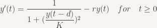


 , and the output
  , must be Numpy arrays (i.e. vectors).
 at any past or present
  using the values of
  if t is inferior to some time
  that marks the start of the integration.
 , it will look for two already computed values
  and
and  at times
  , from which it will deduce

 and
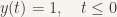
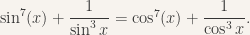
and  , which are the only angles whose sine is equal to the cosine. Now, are there any other solutions ? In the end what is asked is whether the function f is bijective, or not, or just enough ! Let us compute its derivative:
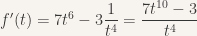
![[-\sqrt[10]{\frac{7}{3}} , +\sqrt[10]{\frac{7}{3}}]](https://s0.wp.com/latex.php?latex=%5B-%5Csqrt%5B10%5D%7B%5Cfrac%7B7%7D%7B3%7D%7D+%2C+%2B%5Csqrt%5B10%5D%7B%5Cfrac%7B7%7D%7B3%7D%7D%5D+&bg=f7f3ee&fg=333333&s=0&c=20201002) . We can now sketch the function:
. We can now sketch the function:
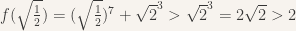
 is placed left to the red zone in the right (see figure). A consequence is that, if u and v belong to the right red zone, then
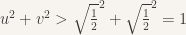
 and for the second
 ![c \in [\frac{ n \pm 2\sqrt{n}}{v}]](https://s0.wp.com/latex.php?latex=c+%5Cin+%5B%5Cfrac%7B+n+%5Cpm+2%5Csqrt%7Bn%7D%7D%7Bv%7D%5D+&bg=f7f3ee&fg=333333&s=0&c=20201002) .
.


 because, in addition, fis and crp regulate themselves !


